Combined Population Health and Service Capacity Model
Contents
Combined Population Health and Service Capacity Model#
Overview#
This notebook contains the code to develop and test the MGSR.
Further details on the development of the population health model can be found here, and the service capacity model can be found here.
#turn warnings off to keep notebook tidy
import warnings
warnings.filterwarnings('ignore')
Import libraries#
import os
import pandas as pd
import numpy as np
import pickle as pkl

from sklearn.linear_model import LinearRegression
from sklearn.ensemble import RandomForestRegressor
from sklearn.ensemble import GradientBoostingRegressor


from sklearn.model_selection import train_test_split
from sklearn.model_selection import GridSearchCV
from sklearn.model_selection import cross_validate
from sklearn.model_selection import RepeatedKFold
from sklearn.metrics import r2_score as r2


import seaborn as sns

import matplotlib.pyplot as plt
%matplotlib inline
plt.style.use('ggplot')
Import data#
dta = pd.read_csv('https://raw.githubusercontent.com/CharlotteJames/ed-forecast/main/data/master_scaled_new_pop.csv',
                  index_col=0)
dta.columns = ['_'.join([c.split('/')[0],c.split('/')[-1]])
               if '/' in c else c for c in dta.columns]
dta.head()
| ccg | month | 111_111_offered | 111_111_answered | amb_sys_made | amb_sys_answered | gp_appt_available | ae_attendances_attendances | population | People | Places | Lives | year | %>65 | %<15 | N>65 | N<15 | |
|---|---|---|---|---|---|---|---|---|---|---|---|---|---|---|---|---|---|
| 0 | 00Q | Jan | 406.655830 | 308.945095 | 310.561801 | 234.716187 | 4568.019766 | 1179.855246 | 14.8942 | 97.2 | 99.7 | 94.4 | 2018 | 14.46402 | 21.763505 | 2.1543 | 3.2415 |
| 1 | 00Q | Feb | 349.933603 | 256.872981 | 261.756435 | 205.298797 | 3910.918344 | 1075.452189 | 14.8942 | 97.2 | 99.7 | 94.4 | 2018 | 14.46402 | 21.763505 | 2.1543 | 3.2415 |
| 2 | 00Q | Mar | 413.247659 | 300.690725 | 303.676215 | 234.716187 | 4051.778545 | 1210.874032 | 14.8942 | 97.2 | 99.7 | 94.4 | 2018 | 14.46402 | 21.763505 | 2.1543 | 3.2415 |
| 3 | 00Q | Apr | 349.608595 | 278.140171 | 264.973181 | 203.677924 | 3974.433001 | 1186.166427 | 14.8942 | 97.2 | 99.7 | 94.4 | 2018 | 14.46402 | 21.763505 | 2.1543 | 3.2415 |
| 4 | 00Q | May | 361.100544 | 284.419492 | 294.361403 | 227.926437 | 4232.385761 | 1299.297713 | 14.8942 | 97.2 | 99.7 | 94.4 | 2018 | 14.46402 | 21.763505 | 2.1543 | 3.2415 |
dta.shape
(1618, 17)
Function to group data#
def group_data(data, features):

    features = ['population', '%>65',
                'People', 'Places',
                'Lives']


    #ensure no identical points in train and test

    grouped = pd.DataFrame()

    for pop, group in data.groupby('population'):

        #if len(group.lives.unique())>1:

            #print('multiple CCG with same population')

        ccg_year = pd.Series(dtype='float64')

        for f in features:

            ccg_year[f] = group[f].unique()[0]

        ccg_year['ae_attendances_attendances']\
        = group.ae_attendances_attendances.mean()


        grouped = grouped.append(ccg_year, ignore_index=True)

    return grouped
Fit Predict Population Health model#
model = RandomForestRegressor(max_depth=7, n_estimators=4,
                              random_state=0)

pophealth_features = ['population', '%>65',
                    'People', 'Places', 'Lives']

grouped = group_data(dta, pophealth_features)

y = grouped['ae_attendances_attendances']

X = grouped[pophealth_features]

cv = RepeatedKFold(n_splits=5, n_repeats=1, random_state=1)

results = pd.DataFrame()


scores_train, scores_test, feat = [],[],[]

for train_index, test_index in cv.split(X, y):

    model.fit(X.iloc[train_index], y.iloc[train_index])

    test = X.iloc[test_index].copy()
    test['ae_predicted'] = model.predict(X.iloc[test_index])

    results = results.append(test, ignore_index=True)
results
| population | %>65 | People | Places | Lives | ae_predicted | |
|---|---|---|---|---|---|---|
| 0 | 14.9084 | 14.565614 | 96.000000 | 99.500 | 94.600000 | 955.021953 |
| 1 | 20.5985 | 19.984465 | 95.500000 | 102.300 | 100.300000 | 803.955255 |
| 2 | 20.9547 | 18.555742 | 101.100000 | 101.600 | 101.300000 | 464.338579 |
| 3 | 21.6203 | 14.128851 | 96.600000 | 96.800 | 94.600000 | 397.401519 |
| 4 | 26.1061 | 15.082682 | 88.600000 | 94.800 | 91.900000 | 684.372748 |
| ... | ... | ... | ... | ... | ... | ... |
| 140 | 137.0653 | 16.343962 | 93.680000 | 98.580 | 91.620000 | 570.391006 |
| 141 | 150.2535 | 13.238627 | 104.566667 | 100.850 | 104.100000 | 382.996087 |
| 142 | 151.1457 | 12.145566 | 101.740000 | 96.820 | 97.540000 | 411.516817 |
| 143 | 181.1249 | 11.599620 | 100.916667 | 97.550 | 99.133333 | 411.516817 |
| 144 | 186.1075 | 19.590720 | 101.100000 | 97.825 | 102.406250 | 385.143687 |
145 rows × 6 columns
Merge with data set#
dta = dta.merge(results[['population','ae_predicted']],\
                left_on='population', right_on='population')
dta
| ccg | month | 111_111_offered | 111_111_answered | amb_sys_made | amb_sys_answered | gp_appt_available | ae_attendances_attendances | population | People | Places | Lives | year | %>65 | %<15 | N>65 | N<15 | ae_predicted | |
|---|---|---|---|---|---|---|---|---|---|---|---|---|---|---|---|---|---|---|
| 0 | 00Q | Jan | 406.655830 | 308.945095 | 310.561801 | 234.716187 | 4568.019766 | 1179.855246 | 14.8942 | 97.2 | 99.7 | 94.4 | 2018 | 14.464020 | 21.763505 | 2.1543 | 3.2415 | 1062.812464 |
| 1 | 00Q | Feb | 349.933603 | 256.872981 | 261.756435 | 205.298797 | 3910.918344 | 1075.452189 | 14.8942 | 97.2 | 99.7 | 94.4 | 2018 | 14.464020 | 21.763505 | 2.1543 | 3.2415 | 1062.812464 |
| 2 | 00Q | Mar | 413.247659 | 300.690725 | 303.676215 | 234.716187 | 4051.778545 | 1210.874032 | 14.8942 | 97.2 | 99.7 | 94.4 | 2018 | 14.464020 | 21.763505 | 2.1543 | 3.2415 | 1062.812464 |
| 3 | 00Q | Apr | 349.608595 | 278.140171 | 264.973181 | 203.677924 | 3974.433001 | 1186.166427 | 14.8942 | 97.2 | 99.7 | 94.4 | 2018 | 14.464020 | 21.763505 | 2.1543 | 3.2415 | 1062.812464 |
| 4 | 00Q | May | 361.100544 | 284.419492 | 294.361403 | 227.926437 | 4232.385761 | 1299.297713 | 14.8942 | 97.2 | 99.7 | 94.4 | 2018 | 14.464020 | 21.763505 | 2.1543 | 3.2415 | 1062.812464 |
| ... | ... | ... | ... | ... | ... | ... | ... | ... | ... | ... | ... | ... | ... | ... | ... | ... | ... | ... |
| 1613 | X2C4Y | Aug | 281.008273 | 253.093792 | 459.652700 | 306.843650 | 3982.517935 | 390.405530 | 44.0337 | 93.3 | 98.3 | 97.6 | 2019 | 17.721427 | 19.239128 | 7.8034 | 8.4717 | 457.428335 |
| 1614 | X2C4Y | Sep | 263.936917 | 240.868701 | 453.078703 | 305.262399 | 4598.750502 | 388.679580 | 44.0337 | 93.3 | 98.3 | 97.6 | 2019 | 17.721427 | 19.239128 | 7.8034 | 8.4717 | 457.428335 |
| 1615 | X2C4Y | Oct | 286.454848 | 254.680032 | 488.348051 | 327.202669 | 5225.611293 | 391.268506 | 44.0337 | 93.3 | 98.3 | 97.6 | 2019 | 17.721427 | 19.239128 | 7.8034 | 8.4717 | 457.428335 |
| 1616 | X2C4Y | Nov | 326.984206 | 276.374619 | 499.497654 | 306.953594 | 4606.948769 | 389.542555 | 44.0337 | 93.3 | 98.3 | 97.6 | 2019 | 17.721427 | 19.239128 | 7.8034 | 8.4717 | 457.428335 |
| 1617 | X2C4Y | Dec | 365.414559 | 334.346359 | 532.917357 | 311.645611 | 4160.472547 | 404.531075 | 44.0337 | 93.3 | 98.3 | 97.6 | 2019 | 17.721427 | 19.239128 | 7.8034 | 8.4717 | 457.428335 |
1618 rows × 18 columns
Combined model#
#capacity utility model
rf1 = RandomForestRegressor(max_depth=5, n_estimators=6,
                            random_state=0)

#combinator
final = LinearRegression()

train, test = train_test_split(dta,random_state=29)

#split training data into two sets
train_0, train_1 = train_test_split(train, train_size=0.75,
                                    random_state=29)


#capacity utility
capacity_features = ['gp_appt_available',
            '111_111_offered', 'amb_sys_answered']
#            '111_111_answered', 'amb_sys_made']

pophealth_features = ['population','%>65',
                    'People', 'Places', 'Lives']

#train capacity modeel

y_0 = train_0['ae_attendances_attendances']
X_0 = train_0[capacity_features]

rf1.fit(X_0,y_0)


#predict

y_pred_cu = rf1.predict(train_1[capacity_features])

print(rf1.score(train_1[capacity_features],
                train_1['ae_attendances_attendances']))

y_pred_ph = train_1['ae_predicted']
0.4519048888936743
X_f = np.vstack([y_pred_cu, y_pred_ph]).T
y_f = train_1['ae_attendances_attendances']

final.fit(X_f,y_f)

final.score(X_f,y_f)
0.8185753379143442
Check performance on held out data#
y_pred_cu = rf1.predict(test[capacity_features])

print(rf1.score(test[capacity_features],
                test['ae_attendances_attendances']))

#y_pred_ph = rf2.predict(test[pophealth_features])

y_pred_ph = test['ae_predicted']

print(r2(test['ae_attendances_attendances'], test['ae_predicted']))

y_pred_final = final.predict(np.vstack([y_pred_cu, y_pred_ph]).T)

#print(r2_score(test['ae_attendances_attendances'], y_pred_final))

print(final.score(np.vstack([y_pred_cu, y_pred_ph]).T,
                  test['ae_attendances_attendances']))
0.4227235191823048
0.7809961790244568
0.8028603990777634
Coefficients#
final.coef_
array([0.33472245, 0.84220157])
Combined model with optimised parameters#
def fit_ph(dta, features, model):

    if 'ae_predicted' in dta.columns:

        dta = dta.drop(['ae_predicted'], axis=1)

    grouped = group_data(dta, features)

    y = grouped['ae_attendances_attendances']

    X = grouped[features]

    # dont set random state so that function can be used in overall cv
    cv = RepeatedKFold(n_splits=5, n_repeats=1, random_state=1)

    results = pd.DataFrame()

    for train_index, test_index in cv.split(X, y):

        model.fit(X.iloc[train_index], y.iloc[train_index])

        test = X.iloc[test_index].copy()

        test['ae_predicted'] = model.predict(X.iloc[test_index])

        results = results.append(test, ignore_index=True)

    dta = dta.merge(results[['population','ae_predicted']],
                    left_on='population', right_on='population')

    return dta
def fit_capacity(dta, features, model):

    y = dta['ae_attendances_attendances']
    X = dta[features]

    model.fit(X,y)

    return model
def fit_combined(train, rf1, m1_features, train_size=7/8):

    final = LinearRegression()

    #split training data into two sets
    train_0, train_1 = train_test_split(train,
                                        train_size=train_size,
                                        random_state=29)

    #train capactiy model

    rf1 = fit_capacity(train_0, m1_features, rf1)


    #predict monthly attendances

    y_pred_1 = rf1.predict(train_1[m1_features])


    #use pre-predicted average attendances

    y_pred_2 = train_1['ae_predicted']

    #final

    X_f = np.vstack([y_pred_1, y_pred_2]).T
    y_f = train_1['ae_attendances_attendances']

    final.fit(X_f,y_f)

    return rf1,final
def cv_combined(dta, rf1, rf2):

    # splitter for cross validation

    cv = RepeatedKFold(n_splits=5, n_repeats=5, random_state=1)

    scores_final, scores_rf1, scores_rf2, coefs = [],[],[],[]

    k=1

    capacity_features = ['gp_appt_available',
            '111_111_offered', 'amb_sys_answered']

    pophealth_features = ['population', '%>65',
                            'People', 'Places', 'Lives']

    dta_pred = pd.DataFrame()

    #fit population health independently to avoid data leakage

    dta = fit_ph(dta, pophealth_features, rf2)

    print(dta.shape)

    for train_index, test_index in cv.split(dta):

        #print(f'\n Split {k} \n')

        train = dta.iloc[train_index]
        test = dta.iloc[test_index]

        #final models
        rf1, final = fit_combined(train, rf1, capacity_features)

        coefs.append(final.coef_)

        #predict on test data

        y_pred_cu = rf1.predict(test[capacity_features])

        scores_rf1.append(rf1.score(test[capacity_features],
                                    test['ae_attendances_attendances']))

        y_pred_ph = test['ae_predicted']

        scores_rf2.append(r2(test['ae_attendances_attendances'],
                             test['ae_predicted']))

        preds = final.predict(np.vstack([y_pred_cu, y_pred_ph]).T)

        scores_final.append(final.score(np.vstack([y_pred_cu, y_pred_ph]).T,
                                        test['ae_attendances_attendances']))

        test_pred = test.copy()
        test_pred['predicted'] = preds
        test_pred['true'] = test['ae_attendances_attendances'].values

        test_pred['iter'] = [k for i in test_pred.index]

        dta_pred = dta_pred.append(test_pred, ignore_index=False)


        k+=1

    return scores_final, scores_rf1, scores_rf2, dta_pred, coefs
#capacity model
rf1 = RandomForestRegressor(max_depth=5, n_estimators=6, random_state=0)

#population health model
rf2 = RandomForestRegressor(max_depth=7, n_estimators=4, random_state=0)

scores_final, scores_rf1, scores_rf2, \
dta_pred, coefs = cv_combined(dta, rf1, rf2)
(1618, 18)
Results for paper#
results=pd.DataFrame()

results['final'] = scores_final
results.describe()
| final | |
|---|---|
| count | 25.000000 |
| mean | 0.793439 |
| std | 0.024965 |
| min | 0.747330 |
| 25% | 0.773945 |
| 50% | 0.792260 |
| 75% | 0.813894 |
| max | 0.837230 |
Coefficient importances#
Mean#
np.mean(coefs, axis=0)
array([0.22809236, 0.85217576])
Std#
np.std(coefs, axis=0)
array([0.06542627, 0.06053951])
Plot#
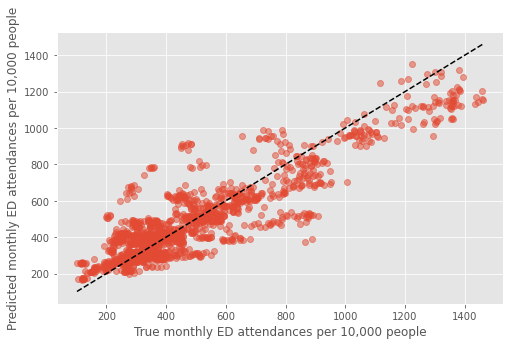
fig,ax = plt.subplots(figsize=(8,5))

mean_pred, true = [],[]

for i in dta_pred.index.unique():

    mean_pred.append(dta_pred.loc[i]['predicted'].mean())
    true.append(dta_pred.loc[i]['true'].mean())

plt.plot(true, mean_pred, 'o', alpha=0.5)

xx = np.arange(min(dta_pred['true']),max(dta_pred['true']))
plt.plot(xx,xx,'k--')

plt.xlabel('True monthly ED attendances per 10,000 people')
plt.ylabel('Predicted monthly ED attendances per 10,000 people')
plt.savefig('true_predicted_combined.png', dpi=300)
plt.show()
Permutation Feature Importance#
def fit_ph_shuffle(dta, features,f, model):

    if 'ae_predicted' in dta.columns:

        dta = dta.drop(['ae_predicted'], axis=1)

    grouped = group_data(dta, features)

    y = grouped['ae_attendances_attendances']

    X = grouped[features]

    X_shuffled = X.copy()

    X_shuffled[f] = np.random.permutation(X[f].values)


    # dont set random state so that function can be used in overall cv
    cv = RepeatedKFold(n_splits=5, n_repeats=1, random_state=1)

    results = pd.DataFrame()

    for train_index, test_index in cv.split(X, y):

        model.fit(X.iloc[train_index], y.iloc[train_index])

        test = X.iloc[test_index].copy()

        test['ae_predicted'] = model.predict(X_shuffled.iloc[test_index])

        results = results.append(test, ignore_index=True)

    dta = dta.merge(results[['population','ae_predicted']],
                    left_on='population', right_on='population')

    return dta
def permeate_feature(dta, f,rf1, rf2):


    shuffled = dta.copy()

    capacity_features = ['gp_appt_available',
            '111_111_offered', 'amb_sys_answered']
#            '111_111_answered', 'amb_sys_made']

    pophealth_features = ['population', '%>65',
                            'People', 'Places', 'Lives']

    if f in capacity_features:

        shuffled[f] = np.random.permutation(dta[f].values)

    else:

        shuffled = fit_ph_shuffle(shuffled, pophealth_features,f, rf2)


    dta = fit_ph(dta, pophealth_features, rf2)

    # splitter for cross validation
    cv = RepeatedKFold(n_splits=5, n_repeats=5, random_state=1)

    #importances = pd.DataFrame()

    shuffled_score, true_score  = [],[]

    #print(f'running for {f} \n')

    for train_index, test_index in cv.split(dta):

        test_shuffled = shuffled.iloc[test_index]

        train = dta.iloc[train_index]
        test = dta.iloc[test_index]


        #final models
        rf1, final = fit_combined(train, rf1, capacity_features)


        #predict on test data

        y_pred_cu = rf1.predict(test[capacity_features])

        y_pred_ph = test['ae_predicted']

        y_pred_cus = rf1.predict(test_shuffled[capacity_features])

        if f in capacity_features:

            y_pred_phs = test['ae_predicted']

        else:

            y_pred_phs = test_shuffled['ae_predicted']


        true_score.append(
            final.score(np.vstack([y_pred_cu, y_pred_ph]).T,\
                                                test['ae_attendances_attendances']))

        shuffled_score.append(
            true_score[-1] - final.score(np.vstack([y_pred_cus, y_pred_phs]).T,\
                                            test['ae_attendances_attendances']))

    #print(f'{f} complete\n')

    return true_score, shuffled_score
def feature_importance_combined(dta, rf1, rf2):

    importances = pd.DataFrame()

    capacity_features = ['gp_appt_available',
            '111_111_offered', 'amb_sys_answered']
    #            '111_111_answered', 'amb_sys_made']

    pophealth_features = ['population', '%>65',
                            'People', 'Places', 'Lives']


    for f in capacity_features + pophealth_features:


        true_score, shuffled_score = permeate_feature(dta, f,rf1, rf2)

        if 'score' in importances.columns:

            importances['score'] = np.mean([importances['score'].values, true_score],axis=0)

        else:

            importances['score'] = true_score

        importances[f] = shuffled_score


    return importances
#set random seed to make results reproducible
np.random.seed(4)

importances = feature_importance_combined(dta, rf1, rf2)
importances.describe()
| score | gp_appt_available | 111_111_offered | amb_sys_answered | population | %>65 | People | Places | Lives | |
|---|---|---|---|---|---|---|---|---|---|
| count | 25.000000 | 25.000000 | 25.000000 | 25.000000 | 25.000000 | 25.000000 | 25.000000 | 25.000000 | 25.000000 |
| mean | 0.793439 | 0.009821 | 0.020091 | 0.048201 | 0.393994 | 0.109398 | 0.070902 | 0.040108 | 0.218843 |
| std | 0.024965 | 0.005905 | 0.009634 | 0.022151 | 0.067007 | 0.018103 | 0.025604 | 0.012660 | 0.036510 |
| min | 0.747330 | -0.000153 | 0.007046 | 0.002438 | 0.311784 | 0.074345 | 0.014080 | 0.015471 | 0.158269 |
| 25% | 0.773945 | 0.004393 | 0.012207 | 0.033947 | 0.333901 | 0.094481 | 0.052257 | 0.033059 | 0.190781 |
| 50% | 0.792260 | 0.011244 | 0.017722 | 0.048973 | 0.381220 | 0.106952 | 0.076336 | 0.041156 | 0.218894 |
| 75% | 0.813894 | 0.014314 | 0.026769 | 0.057536 | 0.445263 | 0.123259 | 0.089431 | 0.045325 | 0.235801 |
| max | 0.837230 | 0.018327 | 0.042118 | 0.096985 | 0.578256 | 0.136224 | 0.111001 | 0.062045 | 0.286407 |
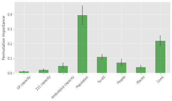
fig,ax = plt.subplots(figsize=(8,5))

importances[importances.columns[1:]].describe().loc['mean'].plot(kind='bar', \
            yerr = importances[importances.columns[1:]].describe().loc['std'],\
                            alpha=0.6, color='g',ax=ax)

plt.ylabel('Permutation Importance', fontsize=12)
plt.tight_layout()

tick_labels = ['GP capacity','111 capacity', 'Ambulance capacity',\
               'Population', '%>65','People', 'Places', 'Lives']

ax.set_xticklabels(tick_labels, rotation=45)

plt.savefig('importance.png', dpi=300)
plt.show()
Train final model on all data and save for forecasting#
def fit_final(dta, rf1, rf2, m1_features, m2_features):


    final = LinearRegression()


    #train capactiy model

    rf1 = fit_capacity(dta, m1_features, rf1)


    #predict monthly attendances

    y_pred_1 = rf1.predict(dta[m1_features])


    grouped = group_data(dta, m2_features)

    y = grouped['ae_attendances_attendances']

    X = grouped[m2_features]

    rf2.fit(X, y)

    y_pred_2 = rf2.predict(dta[m2_features])


    X_f = np.vstack([y_pred_1, y_pred_2]).T
    y_f = dta['ae_attendances_attendances']

    final.fit(X_f,y_f)

    print('Combined training score:',final.score(X_f,y_f))

    return rf1,rf2, final
m1_features = capacity_features
m2_features = pophealth_features

rf1,rf2,final = fit_final(dta, rf1, rf2, m1_features, m2_features)
Combined training score: 0.9181958242731308
with open('stacked_model_scaled.pkl','wb') as f:

    pkl.dump([[rf1,rf2,final], m1_features, m2_features], f)