Outlier analysis
Contents
Outlier analysis#
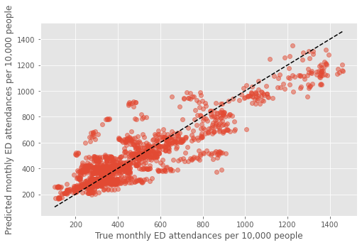
When plotting true vs predicted ED attendances (see Combined Population Health and Service Capacity Model and below) there are two clusters of points that appear to be outliers: Liverpool and Hull.
To understand why these points are outliers in the following we:
fit the model without these points and assess change in performance
investigate the relationship between population health variables and mean monthly ED attendances for these points
#turn warnings off to keep notebook tidy
import warnings
warnings.filterwarnings('ignore')
Import libraries#
import os
import pandas as pd
import numpy as np
import pickle as pkl

from sklearn.linear_model import LinearRegression
from sklearn.ensemble import RandomForestRegressor
from sklearn.ensemble import GradientBoostingRegressor


from sklearn.model_selection import train_test_split
from sklearn.model_selection import GridSearchCV
from sklearn.model_selection import cross_validate
from sklearn.model_selection import RepeatedKFold
from sklearn.metrics import r2_score as r2


import seaborn as sns

import matplotlib.pyplot as plt
%matplotlib inline
plt.style.use('ggplot')
Import data#
dta = pd.read_csv('../data/master_scaled_new_pop.csv', index_col=0)
dta.columns = ['_'.join([c.split('/')[0],c.split('/')[-1]])
               if '/' in c else c for c in dta.columns]
dta.head()
| ccg | month | 111_111_offered | 111_111_answered | amb_sys_made | amb_sys_answered | gp_appt_available | ae_attendances_attendances | population | People | Places | Lives | year | %>65 | %<15 | N>65 | N<15 | |
|---|---|---|---|---|---|---|---|---|---|---|---|---|---|---|---|---|---|
| 0 | 00Q | Jan | 406.655830 | 308.945095 | 310.561801 | 234.716187 | 4568.019766 | 1179.855246 | 14.8942 | 97.2 | 99.7 | 94.4 | 2018 | 14.46402 | 21.763505 | 2.1543 | 3.2415 |
| 1 | 00Q | Feb | 349.933603 | 256.872981 | 261.756435 | 205.298797 | 3910.918344 | 1075.452189 | 14.8942 | 97.2 | 99.7 | 94.4 | 2018 | 14.46402 | 21.763505 | 2.1543 | 3.2415 |
| 2 | 00Q | Mar | 413.247659 | 300.690725 | 303.676215 | 234.716187 | 4051.778545 | 1210.874032 | 14.8942 | 97.2 | 99.7 | 94.4 | 2018 | 14.46402 | 21.763505 | 2.1543 | 3.2415 |
| 3 | 00Q | Apr | 349.608595 | 278.140171 | 264.973181 | 203.677924 | 3974.433001 | 1186.166427 | 14.8942 | 97.2 | 99.7 | 94.4 | 2018 | 14.46402 | 21.763505 | 2.1543 | 3.2415 |
| 4 | 00Q | May | 361.100544 | 284.419492 | 294.361403 | 227.926437 | 4232.385761 | 1299.297713 | 14.8942 | 97.2 | 99.7 | 94.4 | 2018 | 14.46402 | 21.763505 | 2.1543 | 3.2415 |
dta.shape
(1618, 17)
Function to group data#
def group_data(data, features):

    features = ['population','%>65',
                'People', 'Places',
                'Lives']


    #ensure no identical points in train and test

    grouped = pd.DataFrame()

    for pop, group in data.groupby('population'):

        #if len(group.lives.unique())>1:

            #print('multiple CCG with same population')

        ccg_year = pd.Series(dtype='float64')

        for f in features:

            ccg_year[f] = group[f].unique()[0]

        ccg_year['ae_attendances_attendances']\
        = group.ae_attendances_attendances.mean()


        grouped = grouped.append(ccg_year, ignore_index=True)

    return grouped
Functions to fit model#
def fit_ph(dta, features, model):

    if 'ae_predicted' in dta.columns:

        dta = dta.drop(['ae_predicted'], axis=1)

    grouped = group_data(dta, features)

    y = grouped['ae_attendances_attendances']

    X = grouped[features]

    # dont set random state so that function can be used in overall cv
    cv = RepeatedKFold(n_splits=5, n_repeats=1, random_state=1)

    results = pd.DataFrame()

    for train_index, test_index in cv.split(X, y):

        model.fit(X.iloc[train_index], y.iloc[train_index])

        test = X.iloc[test_index].copy()

        test['ae_predicted'] = model.predict(X.iloc[test_index])

        results = results.append(test, ignore_index=True)

    dta = dta.merge(results[['population','ae_predicted']],
                    left_on='population', right_on='population')

    return dta
def fit_capacity(dta, features, model):

    y = dta['ae_attendances_attendances']
    X = dta[features]

    model.fit(X,y)

    return model
def fit_combined(train, rf1, m1_features, train_size=7/8):

    final = LinearRegression()

    #split training data into two sets
    train_0, train_1 = train_test_split(train,
                                        train_size=train_size,
                                        random_state=29)

    #train capactiy model

    rf1 = fit_capacity(train_0, m1_features, rf1)


    #predict monthly attendances

    y_pred_1 = rf1.predict(train_1[m1_features])


    #use pre-predicted average attendances

    y_pred_2 = train_1['ae_predicted']

    #final

    X_f = np.vstack([y_pred_1, y_pred_2]).T
    y_f = train_1['ae_attendances_attendances']

    final.fit(X_f,y_f)

    return rf1,final
def cv_combined(dta, rf1, rf2):

    # splitter for cross validation

    cv = RepeatedKFold(n_splits=5, n_repeats=5, random_state=1)

    scores_final, scores_rf1, scores_rf2, coefs = [],[],[],[]

    k=1

    capacity_features = ['gp_appt_available',
            '111_111_offered', 'amb_sys_answered']

    pophealth_features = ['population','%>65',
                            'People', 'Places', 'Lives']

    dta_pred = pd.DataFrame()

    #fit population health independently to avoid data leakage

    dta = fit_ph(dta, pophealth_features, rf2)

    print(dta.shape)

    for train_index, test_index in cv.split(dta):

        #print(f'\n Split {k} \n')

        train = dta.iloc[train_index]
        test = dta.iloc[test_index]

        #final models
        rf1, final = fit_combined(train, rf1, capacity_features)

        coefs.append(final.coef_)

        #predict on test data

        y_pred_cu = rf1.predict(test[capacity_features])

        scores_rf1.append(rf1.score(test[capacity_features],
                                    test['ae_attendances_attendances']))

        y_pred_ph = test['ae_predicted']

        scores_rf2.append(r2(test['ae_attendances_attendances'],
                             test['ae_predicted']))

        preds = final.predict(np.vstack([y_pred_cu, y_pred_ph]).T)

        scores_final.append(final.score(np.vstack([y_pred_cu, y_pred_ph]).T,
                                        test['ae_attendances_attendances']))

        test_pred = test.copy()
        test_pred['predicted'] = preds
        test_pred['true'] = test['ae_attendances_attendances'].values

        test_pred['iter'] = [k for i in test_pred.index]

        dta_pred = dta_pred.append(test_pred, ignore_index=False)


        k+=1

    return scores_final, scores_rf1, scores_rf2, dta_pred, coefs
Fit model#
#capacity model
rf1 = RandomForestRegressor(max_depth=5, n_estimators=6, random_state=0)

#population health model
rf2 = RandomForestRegressor(max_depth=7, n_estimators=4, random_state=0)

scores_final, scores_rf1, scores_rf2, \
dta_pred, coefs = cv_combined(dta, rf1, rf2)
(1618, 18)
results=pd.DataFrame()

results['final'] = scores_final
results.describe()
| final | |
|---|---|
| count | 25.000000 |
| mean | 0.793439 |
| std | 0.024965 |
| min | 0.747330 |
| 25% | 0.773945 |
| 50% | 0.792260 |
| 75% | 0.813894 |
| max | 0.837230 |
Coefficient importances#
Mean#
np.mean(coefs, axis=0)
array([0.22809236, 0.85217576])
Std#
np.std(coefs, axis=0)
array([0.06542627, 0.06053951])
Plot#
fig,ax = plt.subplots(figsize=(8,5))

mean_pred, true = [],[]

for i in dta_pred.index.unique():

    mean_pred.append(dta_pred.loc[i]['predicted'].mean())
    true.append(dta_pred.loc[i]['true'].mean())

plt.plot(true, mean_pred, 'o', alpha=0.5)

xx = np.arange(min(dta_pred['true']),max(dta_pred['true']))
plt.plot(xx,xx,'k--')

plt.xlabel('True monthly ED attendances per 10,000 people')
plt.ylabel('Predicted monthly ED attendances per 10,000 people')
plt.savefig('true_predicted_combined.png', dpi=300)
plt.show()
Remove Outliers (Hull and Liverpool)#
dta.loc[dta.ccg=='03F']#.shape
| ccg | month | 111_111_offered | 111_111_answered | amb_sys_made | amb_sys_answered | gp_appt_available | ae_attendances_attendances | population | People | Places | Lives | year | %>65 | %<15 | N>65 | N<15 | |
|---|---|---|---|---|---|---|---|---|---|---|---|---|---|---|---|---|---|
| 168 | 03F | Jan | 311.481539 | 305.050947 | 203.403017 | 139.491600 | 4964.760498 | 711.143509 | 26.0645 | 89.4 | 92.5 | 89.1 | 2018 | 14.961730 | 18.913848 | 3.8997 | 4.9298 |
| 169 | 03F | Feb | 270.177030 | 262.694921 | 192.519618 | 138.454451 | 4406.146291 | 655.226074 | 26.0645 | 89.4 | 92.5 | 89.1 | 2018 | 14.961730 | 18.913848 | 3.8997 | 4.9298 |
| 170 | 03F | Mar | 324.018052 | 300.103371 | 219.041964 | 157.986876 | 4704.252911 | 724.854879 | 26.0645 | 89.4 | 92.5 | 89.1 | 2018 | 14.961730 | 18.913848 | 3.8997 | 4.9298 |
| 171 | 03F | Apr | 323.018901 | 288.461277 | 198.272296 | 140.815550 | 4323.773715 | 734.428053 | 26.0645 | 89.4 | 92.5 | 89.1 | 2018 | 14.961730 | 18.913848 | 3.8997 | 4.9298 |
| 172 | 03F | May | 327.195644 | 293.838257 | 209.814335 | 154.673667 | 4469.757716 | 792.073510 | 26.0645 | 89.4 | 92.5 | 89.1 | 2018 | 14.961730 | 18.913848 | 3.8997 | 4.9298 |
| 173 | 03F | Jun | 282.556443 | 255.916616 | 203.076199 | 151.105340 | 4083.216636 | 750.714573 | 26.0645 | 89.4 | 92.5 | 89.1 | 2018 | 14.961730 | 18.913848 | 3.8997 | 4.9298 |
| 174 | 03F | Jul | 302.757300 | 275.694352 | 221.946649 | 160.854878 | 4051.948052 | 787.776478 | 26.0645 | 89.4 | 92.5 | 89.1 | 2018 | 14.961730 | 18.913848 | 3.8997 | 4.9298 |
| 175 | 03F | Aug | 288.159646 | 271.316522 | 209.142356 | 148.732568 | 3657.810432 | 741.391548 | 26.0645 | 89.4 | 92.5 | 89.1 | 2018 | 14.961730 | 18.913848 | 3.8997 | 4.9298 |
| 176 | 03F | Sep | 287.261039 | 266.293539 | 207.219794 | 149.031041 | 3888.660822 | 711.504153 | 26.0645 | 89.4 | 92.5 | 89.1 | 2018 | 14.961730 | 18.913848 | 3.8997 | 4.9298 |
| 177 | 03F | Oct | 308.517602 | 274.766420 | 216.078918 | 152.209187 | 5052.197433 | 758.004182 | 26.0645 | 89.4 | 92.5 | 89.1 | 2018 | 14.961730 | 18.913848 | 3.8997 | 4.9298 |
| 178 | 03F | Nov | 324.677868 | 283.019362 | 216.404069 | 150.103206 | 4711.273955 | 731.147730 | 26.0645 | 89.4 | 92.5 | 89.1 | 2018 | 14.961730 | 18.913848 | 3.8997 | 4.9298 |
| 179 | 03F | Dec | 377.972185 | 342.993535 | 236.239970 | 162.498977 | 3923.689309 | 739.473230 | 26.0645 | 89.4 | 92.5 | 89.1 | 2018 | 14.961730 | 18.913848 | 3.8997 | 4.9298 |
| 974 | 03F | Jan | 344.789276 | 301.606458 | 217.705038 | 154.083105 | 4738.815832 | 747.909492 | 26.1061 | 88.6 | 94.8 | 91.9 | 2019 | 15.082682 | 18.887923 | 3.9375 | 4.9309 |
| 975 | 03F | Feb | 301.573108 | 263.428320 | 196.843188 | 139.876093 | 4234.221121 | 697.384902 | 26.1061 | 88.6 | 94.8 | 91.9 | 2019 | 15.082682 | 18.887923 | 3.9375 | 4.9309 |
| 976 | 03F | Mar | 320.641333 | 290.592411 | 210.426107 | 149.541453 | 4606.662811 | 757.332577 | 26.1061 | 88.6 | 94.8 | 91.9 | 2019 | 15.082682 | 18.887923 | 3.9375 | 4.9309 |
| 977 | 03F | Apr | 296.839402 | 274.771704 | 223.763269 | 148.965865 | 4179.904314 | 753.233919 | 26.1061 | 88.6 | 94.8 | 91.9 | 2019 | 15.082682 | 18.887923 | 3.9375 | 4.9309 |
| 978 | 03F | May | 295.405325 | 272.455920 | 228.982369 | 150.909284 | 4275.016184 | 796.327295 | 26.1061 | 88.6 | 94.8 | 91.9 | 2019 | 15.082682 | 18.887923 | 3.9375 | 4.9309 |
| 979 | 03F | Jun | 274.488224 | 250.661281 | 224.204661 | 147.489707 | 4119.726807 | 779.511302 | 26.1061 | 88.6 | 94.8 | 91.9 | 2019 | 15.082682 | 18.887923 | 3.9375 | 4.9309 |
| 980 | 03F | Jul | 283.749278 | 252.762370 | 241.566092 | 163.683792 | 4634.012740 | 844.515267 | 26.1061 | 88.6 | 94.8 | 91.9 | 2019 | 15.082682 | 18.887923 | 3.9375 | 4.9309 |
| 981 | 03F | Aug | 281.008273 | 253.093792 | 229.826350 | 153.421825 | 4019.137290 | 793.262877 | 26.1061 | 88.6 | 94.8 | 91.9 | 2019 | 15.082682 | 18.887923 | 3.9375 | 4.9309 |
| 982 | 03F | Sep | 263.936917 | 240.868701 | 226.539352 | 152.631199 | 4537.521882 | 792.496773 | 26.1061 | 88.6 | 94.8 | 91.9 | 2019 | 15.082682 | 18.887923 | 3.9375 | 4.9309 |
| 983 | 03F | Oct | 286.454848 | 254.680032 | 244.174026 | 163.601334 | 5194.839520 | 794.028982 | 26.1061 | 88.6 | 94.8 | 91.9 | 2019 | 15.082682 | 18.887923 | 3.9375 | 4.9309 |
| 984 | 03F | Nov | 326.984206 | 276.374619 | 249.748827 | 153.476797 | 4584.369170 | 774.416707 | 26.1061 | 88.6 | 94.8 | 91.9 | 2019 | 15.082682 | 18.887923 | 3.9375 | 4.9309 |
| 985 | 03F | Dec | 365.414559 | 334.346359 | 266.458679 | 155.822805 | 4166.191043 | 791.424227 | 26.1061 | 88.6 | 94.8 | 91.9 | 2019 | 15.082682 | 18.887923 | 3.9375 | 4.9309 |
dta.loc[dta.ccg=='99A']
| ccg | month | 111_111_offered | 111_111_answered | amb_sys_made | amb_sys_answered | gp_appt_available | ae_attendances_attendances | population | People | Places | Lives | year | %>65 | %<15 | N>65 | N<15 | |
|---|---|---|---|---|---|---|---|---|---|---|---|---|---|---|---|---|---|
| 665 | 99A | Jan | 406.655830 | 308.945095 | 310.561801 | 234.716187 | 4713.508510 | 897.064351 | 49.4814 | 87.8 | 98.6 | 91.4 | 2018 | 14.673797 | 16.419099 | 7.2608 | 8.1244 |
| 666 | 99A | Feb | 349.933603 | 256.872981 | 261.756435 | 205.298797 | 4152.772557 | 776.049182 | 49.4814 | 87.8 | 98.6 | 91.4 | 2018 | 14.673797 | 16.419099 | 7.2608 | 8.1244 |
| 667 | 99A | Mar | 413.247659 | 300.690725 | 303.676215 | 234.716187 | 4405.453362 | 897.751478 | 49.4814 | 87.8 | 98.6 | 91.4 | 2018 | 14.673797 | 16.419099 | 7.2608 | 8.1244 |
| 668 | 99A | Apr | 349.608595 | 278.140171 | 264.973181 | 203.677924 | 4046.510406 | 848.116666 | 49.4814 | 87.8 | 98.6 | 91.4 | 2018 | 14.673797 | 16.419099 | 7.2608 | 8.1244 |
| 669 | 99A | May | 361.100544 | 284.419492 | 294.361403 | 227.926437 | 4299.837919 | 921.396727 | 49.4814 | 87.8 | 98.6 | 91.4 | 2018 | 14.673797 | 16.419099 | 7.2608 | 8.1244 |
| 670 | 99A | Jun | 328.551827 | 254.368753 | 281.106911 | 220.213747 | 4020.460213 | 863.698279 | 49.4814 | 87.8 | 98.6 | 91.4 | 2018 | 14.673797 | 16.419099 | 7.2608 | 8.1244 |
| 671 | 99A | Jul | 339.766686 | 248.935286 | 297.869823 | 235.572458 | 4166.899077 | 883.604748 | 49.4814 | 87.8 | 98.6 | 91.4 | 2018 | 14.673797 | 16.419099 | 7.2608 | 8.1244 |
| 672 | 99A | Aug | 300.161546 | 239.420469 | 274.165073 | 213.851091 | 3994.591907 | 803.837402 | 49.4814 | 87.8 | 98.6 | 91.4 | 2018 | 14.673797 | 16.419099 | 7.2608 | 8.1244 |
| 673 | 99A | Sep | 302.357433 | 244.118501 | 269.156617 | 209.471816 | 3998.512572 | 822.511085 | 49.4814 | 87.8 | 98.6 | 91.4 | 2018 | 14.673797 | 16.419099 | 7.2608 | 8.1244 |
| 674 | 99A | Oct | 326.893453 | 255.939625 | 299.024018 | 230.861925 | 5037.165480 | 880.753980 | 49.4814 | 87.8 | 98.6 | 91.4 | 2018 | 14.673797 | 16.419099 | 7.2608 | 8.1244 |
| 675 | 99A | Nov | 336.222849 | 265.783617 | 283.988231 | 216.549073 | 4756.312473 | 885.047634 | 49.4814 | 87.8 | 98.6 | 91.4 | 2018 | 14.673797 | 16.419099 | 7.2608 | 8.1244 |
| 676 | 99A | Dec | 397.682693 | 323.605872 | 285.202845 | 228.236861 | 3660.668453 | 866.365463 | 49.4814 | 87.8 | 98.6 | 91.4 | 2018 | 14.673797 | 16.419099 | 7.2608 | 8.1244 |
| 1496 | 99A | Jan | 347.450401 | 275.144606 | 276.797526 | 223.661852 | 4526.771488 | 472.981912 | 49.8945 | 86.5 | 98.9 | 90.0 | 2019 | 14.761747 | 16.561144 | 7.3653 | 8.2631 |
| 1497 | 99A | Feb | 311.886541 | 253.462976 | 247.201714 | 198.606966 | 4108.909800 | 448.696189 | 49.8945 | 86.5 | 98.9 | 90.0 | 2019 | 14.761747 | 16.561144 | 7.3653 | 8.2631 |
| 1498 | 99A | Mar | 317.916884 | 277.724317 | 259.446256 | 208.037004 | 4323.622844 | 484.572288 | 49.8945 | 86.5 | 98.9 | 90.0 | 2019 | 14.761747 | 16.561144 | 7.3653 | 8.2631 |
| 1499 | 99A | Apr | 326.639691 | 286.837872 | 261.284595 | 207.529233 | 4029.622503 | 452.711060 | 49.8945 | 86.5 | 98.9 | 90.0 | 2019 | 14.761747 | 16.561144 | 7.3653 | 8.2631 |
| 1500 | 99A | May | 331.225629 | 287.382197 | 263.684592 | 207.844258 | 4248.845063 | 472.811793 | 49.8945 | 86.5 | 98.9 | 90.0 | 2019 | 14.761747 | 16.561144 | 7.3653 | 8.2631 |
| 1501 | 99A | Jun | 317.485312 | 265.251500 | 264.530186 | 214.654611 | 3944.322521 | 456.905591 | 49.8945 | 86.5 | 98.9 | 90.0 | 2019 | 14.761747 | 16.561144 | 7.3653 | 8.2631 |
| 1502 | 99A | Jul | 322.049866 | 257.638726 | 277.674209 | 231.568576 | 4483.259678 | 481.824249 | 49.8945 | 86.5 | 98.9 | 90.0 | 2019 | 14.761747 | 16.561144 | 7.3653 | 8.2631 |
| 1503 | 99A | Aug | 324.528488 | 265.552822 | 267.709456 | 221.390352 | 3803.124593 | 449.495876 | 49.8945 | 86.5 | 98.9 | 90.0 | 2019 | 14.761747 | 16.561144 | 7.3653 | 8.2631 |
| 1504 | 99A | Sep | 310.420752 | 244.724616 | 261.819309 | 216.466007 | 4205.172915 | 465.664953 | 49.8945 | 86.5 | 98.9 | 90.0 | 2019 | 14.761747 | 16.561144 | 7.3653 | 8.2631 |
| 1505 | 99A | Oct | 333.859773 | 254.714923 | 279.120839 | 233.448366 | 5226.427763 | 922.338855 | 49.8945 | 86.5 | 98.9 | 90.0 | 2019 | 14.761747 | 16.561144 | 7.3653 | 8.2631 |
| 1506 | 99A | Nov | 391.947023 | 275.362336 | 291.417194 | 246.513632 | 4657.186664 | 884.746174 | 49.8945 | 86.5 | 98.9 | 90.0 | 2019 | 14.761747 | 16.561144 | 7.3653 | 8.2631 |
| 1507 | 99A | Dec | 437.959979 | 313.303730 | 304.082460 | 255.023464 | 4029.702673 | 861.508904 | 49.8945 | 86.5 | 98.9 | 90.0 | 2019 | 14.761747 | 16.561144 | 7.3653 | 8.2631 |
hull = dta.loc[(dta.ccg=='03F') & (dta.year==2018)]
liv = dta.loc[(dta.ccg=='99A') & (dta.year==2019)]
dta2 = dta.drop(hull.index)
dta2 = dta2.drop(liv.index)

scores_final, scores_rf1, scores_rf2, \
dta_pred, coefs = cv_combined(dta2, rf1, rf2)
(1594, 18)
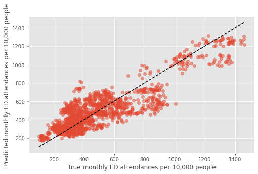
Results#
results=pd.DataFrame()

results['final'] = scores_final
results.describe()
| final | |
|---|---|
| count | 25.000000 |
| mean | 0.764970 |
| std | 0.030494 |
| min | 0.699989 |
| 25% | 0.749633 |
| 50% | 0.769406 |
| 75% | 0.791617 |
| max | 0.807528 |
Plot#
fig,ax = plt.subplots(figsize=(8,5))

mean_pred, true = [],[]

for i in dta_pred.index.unique():

    mean_pred.append(dta_pred.loc[i]['predicted'].mean())
    true.append(dta_pred.loc[i]['true'].mean())

plt.plot(true, mean_pred, 'o', alpha=0.5)

xx = np.arange(min(dta_pred['true']),max(dta_pred['true']))
plt.plot(xx,xx,'k--')

plt.xlabel('True monthly ED attendances per 10,000 people')
plt.ylabel('Predicted monthly ED attendances per 10,000 people')
plt.savefig('true_predicted_combined.png', dpi=300)
plt.show()
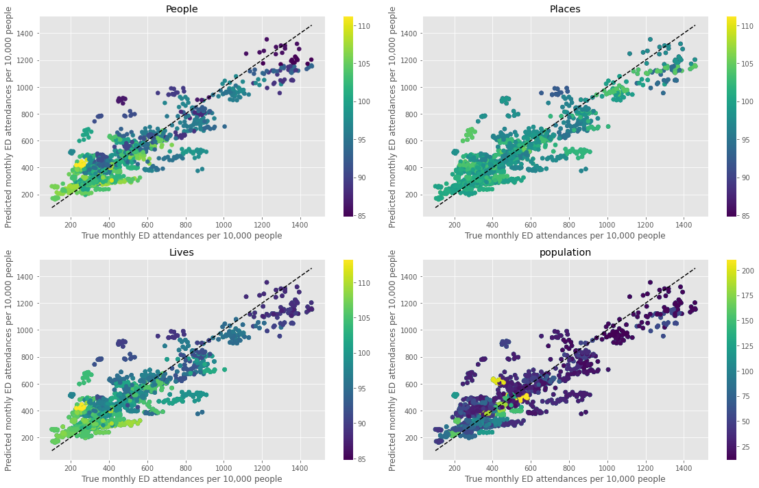
Plot coloured by each grouped feature#
features = ['population',
            'People', 'Places', 'Lives', '%>65']

grouped = group_data(dta, features)
grouped
| population | %>65 | People | Places | Lives | ae_attendances_attendances | |
|---|---|---|---|---|---|---|
| 0 | 11.6159 | 27.037078 | 94.800000 | 103.700000 | 95.400000 | 1024.414811 |
| 1 | 11.6571 | 27.403900 | 97.400000 | 104.200000 | 96.300000 | 1059.954877 |
| 2 | 13.9240 | 20.451020 | 84.800000 | 98.500000 | 88.500000 | 1362.970411 |
| 3 | 13.9305 | 20.388356 | 85.800000 | 97.600000 | 88.000000 | 1275.055932 |
| 4 | 14.8942 | 14.464020 | 97.200000 | 99.700000 | 94.400000 | 1111.556848 |
| ... | ... | ... | ... | ... | ... | ... |
| 140 | 186.1075 | 19.590720 | 101.100000 | 97.825000 | 102.406250 | 371.421898 |
| 141 | 200.8447 | 10.076840 | 103.657143 | 96.357143 | 94.585714 | 442.040841 |
| 142 | 202.9265 | 10.182751 | 103.842857 | 96.414286 | 94.585714 | 429.112528 |
| 143 | 209.5479 | 12.973740 | 105.755556 | 95.666667 | 97.155556 | 554.092008 |
| 144 | 210.8074 | 13.227097 | 104.644444 | 96.000000 | 97.033333 | 510.184272 |
145 rows × 6 columns
scores_final, scores_rf1, scores_rf2, \
dta_pred, coefs = cv_combined(dta, rf1, rf2)
(1618, 18)
fig,ax_list = plt.subplots(2,2, figsize=(16,10))

mean_pred, true, col = [],[],[]

feats = ['People','Places','Lives','population']
# convert range into

for i,f in enumerate(feats):

    ax = ax_list.flatten()[i]

    for i in dta_pred.index.unique():

        mean_pred.append(dta_pred.loc[i]['predicted'].mean())
        true.append(dta_pred.loc[i]['true'].mean())
        col.append(dta_pred.loc[i][f].mean())


    p = ax.scatter(true, mean_pred,  c = col, cmap='viridis')

    xx = np.arange(min(dta_pred['true']),max(dta_pred['true']))
    ax.plot(xx,xx,'k--')

    ax.set_xlabel('True monthly ED attendances per 10,000 people')
    ax.set_ylabel('Predicted monthly ED attendances per 10,000 people')
    ax.set_title(f'{f}')

    fig.colorbar(p, pad=0.05, ax=ax)

plt.tight_layout()

plt.savefig('true_predicted_grouped.png', dpi=300)
plt.show()
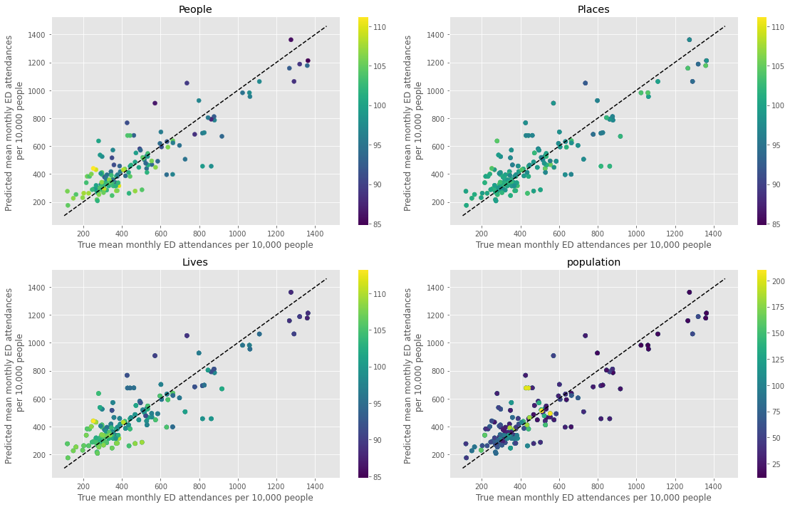
Plot predicted mean monthly attendances#
fig,ax_list = plt.subplots(2,2, figsize=(16,10))

mean_pred, true, col = [],[],[]

feats = ['People','Places','Lives','population']
# convert range into

for i,f in enumerate(feats):

    ax = ax_list.flatten()[i]

    for c in dta_pred.ccg.unique():

        for y in dta_pred.year.unique():

            mean_pred.append(dta_pred.loc[(dta_pred.ccg==c) & (dta_pred.year==y)]['ae_predicted'].mean())
            true.append(dta_pred.loc[(dta_pred.ccg==c) & (dta_pred.year==y)]['true'].mean())
            col.append(dta_pred.loc[(dta_pred.ccg==c) & (dta_pred.year==y)][f].mean())


    p = ax.scatter(true, mean_pred,  c = col, cmap='viridis')

    xx = np.arange(min(dta_pred['true']),max(dta_pred['true']))
    ax.plot(xx,xx,'k--')

    ax.set_xlabel('True mean monthly ED attendances per 10,000 people')
    ax.set_ylabel('Predicted mean monthly ED attendances \n per 10,000 people')
    ax.set_title(f'{f}')

    fig.colorbar(p, pad=0.05, ax=ax)

plt.tight_layout()

plt.savefig('true_predicted_mean.png', dpi=300)
plt.show()
Summary#
From the above figure, the outliers points have low values of ‘People’ and ‘Lives’. When fitting the population health model, as variables only change annually there are fewer datapoints (145 total).
Looking at the ‘Lives’ panel in the final figure, if the model is trained on a subsection of the data that contains data points with low values of this variable (darker points) but high mean monthly ED attendances (cluster in top right), it will predict that an unseen datapoint with a low value of Lives has a high number of ED attendances (dark point centre top – that’s Hull).
As the MGSR assigns a higher weight to the population health model, if the prediction of the population health model isn’t as good for a given ccg, that ccg will be an outlier overall. Model perfomance would improve with an increased amount of data in the future.