Separating Capacity and Utility#

Overview#

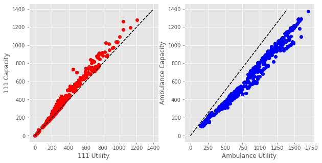
The capacity and utility features are highly correlated (see below). This can affect overall model performance and feature importances.

To understand the extent of this effect we fit separate models to capacity and utility features, and compare performance.

Capacity features: 111 calls offered, Ambulance answered, GP appointments available
Utility features: 111 calls answered, Ambulance made

#turn warnings off to keep notebook tidy
import warnings
warnings.filterwarnings('ignore')

Import libraries#

import os
import pandas as pd
import numpy as np

from sklearn.ensemble import RandomForestRegressor
from sklearn.ensemble import GradientBoostingRegressor
from sklearn.linear_model import LinearRegression


from sklearn.model_selection import train_test_split
from sklearn.pipeline import make_pipeline
from sklearn.preprocessing import StandardScaler

from sklearn.model_selection import cross_validate
from sklearn.model_selection import RepeatedKFold

import matplotlib.pyplot as plt
%matplotlib inline
plt.style.use('ggplot')

Import data#

dta = pd.read_csv('https://raw.githubusercontent.com/CharlotteJames/ed-forecast/main/data/master_scaled_new.csv',
                  index_col=0)

dta.columns = ['_'.join([c.split('/')[0],c.split('/')[-1]]) 
               if '/' in c else c for c in dta.columns]

dta.ccg.unique().shape

(74,)

Feature correlations#

fig,ax_list = plt.subplots(1,2, figsize = (10,5))

xx = np.arange(0,140)*10

ax = ax_list[0]

ax.plot(dta['111_111_answered'].values, dta['111_111_offered'].values, 'ro')
ax.set_xlabel('111 Utility')
ax.set_ylabel('111 Capacity')
ax.plot(xx,xx, 'k--')

ax = ax_list[1]

ax.plot(dta['amb_sys_made'].values, dta['amb_sys_answered'].values, 'bo')
ax.set_xlabel('Ambulance Utility')
ax.set_ylabel('Ambulance Capacity')
ax.plot(xx,xx,'k--')

plt.show()

Add random feature#

# Adding random features

rng = np.random.RandomState(0)
rand_var = rng.rand(dta.shape[0])
dta['rand1'] = rand_var

dta.shape

(1618, 14)

Fitting function#

def fit_model(dta, model, features):
    
    
    y = dta['ae_attendances_attendances']
    X = dta[features]
    
    #cross validate to get errors on performance and coefficients
    cv_model = cross_validate(model, X,y, 
                            cv=RepeatedKFold(n_splits=5, n_repeats=5,
                                             random_state=0),
                            return_estimator=True, 
                              return_train_score=True, n_jobs=2)
    
    clf = model.fit(X, y)

    
    return cv_model

Utility Model#

features = ['111_111_answered', 'amb_sys_made', 'rand1']

Linear Regression#

model = LinearRegression()

results = fit_model(dta,model,features)

Performance#

res=pd.DataFrame()
res['test_score'] = results['test_score']
res['train_score'] = results['train_score']

res.describe()

	test_score	train_score
count	25.000000	25.000000
mean	0.083855	0.089997
std	0.023747	0.004965
min	0.046392	0.074933
25%	0.072955	0.087500
50%	0.084371	0.089937
75%	0.096630	0.093126
max	0.161442	0.100655

Coefficients#

coefs = pd.DataFrame(
   [model.coef_
    for model in results['estimator']],
   columns=features
)

coefs.describe()

	111_111_answered	amb_sys_made	rand1
count	25.000000	25.000000	25.000000
mean	0.388187	-0.136642	-3.708228
std	0.016808	0.007403	12.305010
min	0.339519	-0.149784	-25.111645
25%	0.380248	-0.142231	-9.562033
50%	0.388083	-0.135624	-4.667144
75%	0.395557	-0.132207	4.321049
max	0.427379	-0.121675	19.347927

Random Forest#

model = RandomForestRegressor()

results = fit_model(dta,model,features)

Performance#

res=pd.DataFrame()
res['test_score'] = results['test_score']
res['train_score'] = results['train_score']

res.describe()

	test_score	train_score
count	25.000000	25.000000
mean	0.236590	0.894535
std	0.066466	0.003297
min	0.112391	0.888562
25%	0.197762	0.892035
50%	0.243202	0.894518
75%	0.279811	0.897373
max	0.331515	0.901216

Coefficients#

coefs = pd.DataFrame(
   [model.feature_importances_
    for model in results['estimator']],
   columns=features
)

coefs.describe()

	111_111_answered	amb_sys_made	rand1
count	25.000000	25.000000	25.000000
mean	0.207987	0.440134	0.351879
std	0.005848	0.009332	0.009254
min	0.195764	0.424368	0.326420
25%	0.205005	0.433463	0.347748
50%	0.207886	0.440542	0.351117
75%	0.211373	0.444091	0.357582
max	0.221227	0.465251	0.368511

Gradient Boosted Trees#

model = GradientBoostingRegressor()

results = fit_model(dta,model,features)

Performance#

res=pd.DataFrame()
res['test_score'] = results['test_score']
res['train_score'] = results['train_score']

res.describe()

	test_score	train_score
count	25.000000	25.000000
mean	0.337244	0.493172
std	0.038370	0.009531
min	0.246938	0.475122
25%	0.305860	0.488163
50%	0.347487	0.493584
75%	0.369488	0.497437
max	0.387623	0.512314

Coefficients#

coefs = pd.DataFrame(
   [model.feature_importances_
    for model in results['estimator']],
   columns=features
)

coefs.describe()

	111_111_answered	amb_sys_made	rand1
count	25.000000	25.000000	25.000000
mean	0.196963	0.671507	0.131530
std	0.009310	0.014289	0.010002
min	0.180775	0.638809	0.114408
25%	0.190780	0.660383	0.124134
50%	0.197679	0.673083	0.130621
75%	0.204245	0.681347	0.137798
max	0.211885	0.697861	0.149508

Summary#

Linear regression performs poorly, with an \(R^2\) < 0.1

Random Forest overfits to the training data, and the random variable is comparatively important

Gradient boosted trees performs best and does not overfit. The random variable is ranked lowest.

Capacity Model#

features = ['gp_appt_available',
            '111_111_offered', 'amb_sys_answered', 'rand1']

Linear Regression#

model = LinearRegression()

results = fit_model(dta,model,features)

Performance#

res=pd.DataFrame()
res['test_score'] = results['test_score']
res['train_score'] = results['train_score']

res.describe()

	test_score	train_score
count	25.000000	25.000000
mean	0.102073	0.108765
std	0.026177	0.005678
min	0.052969	0.092187
25%	0.088854	0.105822
50%	0.104882	0.108816
75%	0.113505	0.112577
max	0.188438	0.122830

Coefficients#

coefs = pd.DataFrame(
   [model.coef_
    for model in results['estimator']],
   columns=features
)

coefs.describe()

	gp_appt_available	111_111_offered	amb_sys_answered	rand1
count	25.000000	25.000000	25.000000	25.000000
mean	0.009613	0.481967	-0.108094	-1.058362
std	0.003273	0.012217	0.009119	12.414753
min	0.002709	0.451203	-0.125017	-21.694177
25%	0.007641	0.478179	-0.115796	-7.409371
50%	0.010039	0.481001	-0.107188	-2.177476
75%	0.011166	0.487988	-0.101752	8.037063
max	0.016756	0.509044	-0.089849	21.684858

Random Forest#

model = RandomForestRegressor()

results = fit_model(dta,model,features)

Performance#

res=pd.DataFrame()
res['test_score'] = results['test_score']
res['train_score'] = results['train_score']

res.describe()

	test_score	train_score
count	25.000000	25.000000
mean	0.380144	0.914196
std	0.064979	0.003352
min	0.232751	0.908657
25%	0.335715	0.912098
50%	0.389321	0.913890
75%	0.425642	0.916405
max	0.510369	0.921425

Coefficients#

coefs = pd.DataFrame(
   [model.feature_importances_
    for model in results['estimator']],
   columns=features
)

coefs.describe()

	gp_appt_available	111_111_offered	amb_sys_answered	rand1
count	25.000000	25.000000	25.000000	25.000000
mean	0.239598	0.189017	0.401606	0.169778
std	0.005962	0.011403	0.013790	0.007099
min	0.229238	0.167500	0.378487	0.150998
25%	0.234416	0.181186	0.392606	0.164699
50%	0.239503	0.187306	0.400261	0.170325
75%	0.243710	0.197662	0.410551	0.173957
max	0.251220	0.216889	0.437289	0.183189

Gradient Boosted Trees#

model = GradientBoostingRegressor()

results = fit_model(dta,model,features)

Performance#

res=pd.DataFrame()
res['test_score'] = results['test_score']
res['train_score'] = results['train_score']

res.describe()

	test_score	train_score
count	25.000000	25.000000
mean	0.401899	0.565627
std	0.050106	0.009447
min	0.310316	0.549283
25%	0.369650	0.556523
50%	0.405141	0.567855
75%	0.437094	0.573057
max	0.491685	0.584443

Coefficients#

coefs = pd.DataFrame(
   [model.feature_importances_
    for model in results['estimator']],
   columns=features
)

coefs.describe()

	gp_appt_available	111_111_offered	amb_sys_answered	rand1
count	25.000000	25.000000	25.000000	25.000000
mean	0.161047	0.182368	0.598112	0.058473
std	0.011149	0.014722	0.016180	0.007970
min	0.136198	0.153994	0.561232	0.043424
25%	0.156540	0.175966	0.589252	0.053474
50%	0.161440	0.180021	0.599186	0.057511
75%	0.168531	0.189533	0.608987	0.062670
max	0.184913	0.227816	0.625746	0.075962

Summary#

Linear regression again performs poorly.

Random Forest overfits to the training data, but the random variable is ranked lowest.

Gradient boosted trees performs best and does not overfit. The random variable is ranked lowest.

Forecasting Long Term ED Demand

Separating Capacity and Utility

Contents

Separating Capacity and Utility#

Overview#

Import libraries#

Import data#

Feature correlations#

Add random feature#

Fitting function#

Utility Model#

Linear Regression#

Performance#

Coefficients#

Random Forest#

Performance#

Coefficients#

Gradient Boosted Trees#

Performance#

Coefficients#

Summary#

Capacity Model#

Linear Regression#

Performance#

Coefficients#

Random Forest#

Performance#

Coefficients#

Gradient Boosted Trees#

Performance#

Coefficients#

Summary#