Forecasting Future ED Demand
Contents
Forecasting Future ED Demand#
Overview#
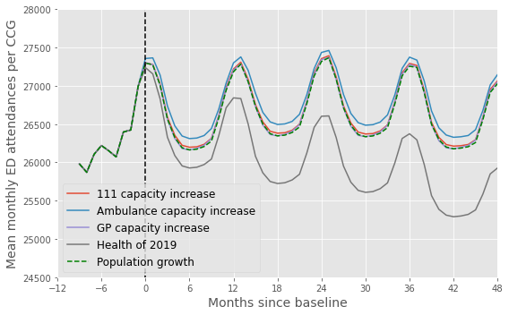
This notebook contains the code to forecast future ED demand under 4 different scenarios:
‘do nothing’: population grows but population health and health service capacity reamin unchanged
Increase 111 capacity by 10% in 2020
Increase 999 capacity by 10% in 2020
Increase GP capacity by 10% in 2020
If population health measures (People, Places, Lives) are less than the 2019 average, increase them by 0.2 points per year until they reach the 2019 average.
#turn warnings off to keep notebook tidy
import warnings
warnings.filterwarnings('ignore')
Import libraries#
import os
import pandas as pd
import numpy as np
import pickle as pkl

from sklearn.linear_model import LinearRegression
from sklearn.ensemble import RandomForestRegressor
from sklearn.ensemble import GradientBoostingRegressor


import seaborn as sns
import matplotlib.pyplot as plt
%matplotlib inline
plt.style.use('ggplot')
Import trained models#
with open('stacked_model_scaled.pkl','rb') as f:

    models, m1_features, m2_features = pkl.load(f)
NB if running notebook on colab the above code wont work. Instead, run the following cell:
%run stacked_model.ipynb

models = [rf1,rf2,final]
0.4519048888936743
0.4227235191823048
0.7809961790244568
0.8028603990777634
(1618, 18)
Combined training score: 0.9181958242731308
Import population forecasts#
population = pd.read_csv('https://raw.githubusercontent.com/CharlotteJames/ed-forecast/main/data/pop_forecasts_scaled_new.csv',
                  index_col=0)
population
| 2018 | 2019 | 2020 | 2021 | 2022 | 2023 | 2024 | 2025 | 2026 | 2027 | ... | 2035 | 2036 | 2037 | 2038 | 2039 | 2040 | 2041 | 2042 | 2043 | ccg | |
|---|---|---|---|---|---|---|---|---|---|---|---|---|---|---|---|---|---|---|---|---|---|
| 0 | 200.8447 | 202.9265 | 204.7996 | 206.5125 | 208.0446 | 209.3943 | 210.5565 | 211.5642 | 212.5387 | 213.4931 | ... | 221.2491 | 222.2393 | 223.2383 | 224.2422 | 225.2318 | 226.1957 | 227.1281 | 228.0246 | 228.8859 | A3A8R |
| 1 | 209.5479 | 210.8074 | 211.8850 | 212.8265 | 213.6216 | 214.2545 | 214.7215 | 215.0593 | 215.4030 | 215.7479 | ... | 219.0375 | 219.4856 | 219.9439 | 220.4162 | 220.8884 | 221.3468 | 221.7894 | 222.2189 | 222.6387 | W2U3Z |
| 2 | 149.4905 | 150.2535 | 150.9484 | 151.6046 | 152.1883 | 152.6870 | 153.1002 | 153.4384 | 153.7346 | 154.0150 | ... | 156.6288 | 157.0287 | 157.4507 | 157.8919 | 158.3365 | 158.7785 | 159.2128 | 159.6398 | 160.0604 | 36L |
| 3 | 181.1249 | 182.6084 | 183.9507 | 185.1905 | 186.3272 | 187.3571 | 188.2697 | 189.0749 | 189.8431 | 190.5932 | ... | 197.0201 | 197.8779 | 198.7388 | 199.6013 | 200.4489 | 201.2717 | 202.0611 | 202.8162 | 203.5407 | 72Q |
| 4 | 149.8001 | 151.1457 | 152.3376 | 153.3887 | 154.3113 | 155.1054 | 155.7686 | 156.3214 | 156.8646 | 157.4020 | ... | 161.9110 | 162.4828 | 163.0498 | 163.6149 | 164.1693 | 164.7041 | 165.2164 | 165.7083 | 166.1828 | 93C |
| ... | ... | ... | ... | ... | ... | ... | ... | ... | ... | ... | ... | ... | ... | ... | ... | ... | ... | ... | ... | ... | ... |
| 76 | 21.5133 | 21.6203 | 21.6898 | 21.7321 | 21.7657 | 21.8065 | 21.8544 | 21.9101 | 21.9739 | 22.0439 | ... | 22.4638 | 22.5006 | 22.5295 | 22.5486 | 22.5715 | 22.5996 | 22.6308 | 22.6632 | 22.6963 | 10R |
| 77 | 48.9709 | 49.2387 | 49.4684 | 49.6714 | 49.8482 | 50.0060 | 50.1449 | 50.2665 | 50.3747 | 50.4696 | ... | 50.9995 | 51.0625 | 51.1297 | 51.1994 | 51.2754 | 51.3581 | 51.4457 | 51.5383 | 51.6351 | 15A |
| 78 | 56.8210 | 57.4154 | 57.9778 | 58.5240 | 59.0612 | 59.5859 | 60.1019 | 60.6047 | 61.0936 | 61.5704 | ... | 64.7377 | 65.0715 | 65.3987 | 65.7217 | 66.0425 | 66.3625 | 66.6815 | 66.9986 | 67.3133 | 11N |
| 79 | 55.9399 | 56.3600 | 56.7726 | 57.1821 | 57.5799 | 57.9658 | 58.3368 | 58.6904 | 59.0312 | 59.3577 | ... | 61.6103 | 61.8668 | 62.1228 | 62.3799 | 62.6334 | 62.8819 | 63.1262 | 63.3669 | 63.6048 | 11X |
| 80 | 85.8852 | 86.5409 | 87.1659 | 87.7879 | 88.3855 | 88.9617 | 89.5148 | 90.0372 | 90.5408 | 91.0223 | ... | 94.3408 | 94.7170 | 95.0941 | 95.4763 | 95.8582 | 96.2381 | 96.6183 | 96.9977 | 97.3744 | 70F |
81 rows × 27 columns
pop_g65 = pd.read_csv('https://raw.githubusercontent.com/CharlotteJames/ed-forecast/main/data/g65_forecasts.csv',index_col=0)
pop_g65
| 2018 | 2019 | 2020 | 2021 | 2022 | 2023 | 2024 | 2025 | 2026 | 2027 | ... | 2035 | 2036 | 2037 | 2038 | 2039 | 2040 | 2041 | 2042 | 2043 | ccg | |
|---|---|---|---|---|---|---|---|---|---|---|---|---|---|---|---|---|---|---|---|---|---|
| 0 | 20.2388 | 20.6635 | 21.0618 | 21.5045 | 22.0027 | 22.5320 | 23.0877 | 23.6772 | 24.2807 | 24.8923 | ... | 30.3201 | 30.9727 | 31.5959 | 32.1724 | 32.7359 | 33.3015 | 33.8719 | 34.4506 | 35.0449 | A3A8R |
| 1 | 27.1862 | 27.8837 | 28.5918 | 29.3262 | 30.0403 | 30.8135 | 31.5979 | 32.4221 | 33.2414 | 34.1069 | ... | 41.0640 | 41.8279 | 42.5907 | 43.3212 | 44.0126 | 44.6750 | 45.3063 | 45.9144 | 46.5156 | W2U3Z |
| 2 | 19.5244 | 19.8915 | 20.2332 | 20.6187 | 21.0258 | 21.4313 | 21.8943 | 22.3840 | 22.9167 | 23.4920 | ... | 28.2659 | 28.7972 | 29.3256 | 29.8007 | 30.2389 | 30.6803 | 31.0964 | 31.5105 | 31.9304 | 36L |
| 3 | 21.0098 | 21.3213 | 21.6398 | 22.0230 | 22.4571 | 22.9487 | 23.4649 | 24.0559 | 24.6942 | 25.3515 | ... | 30.7090 | 31.2815 | 31.8039 | 32.2985 | 32.7302 | 33.1674 | 33.6041 | 34.0586 | 34.5384 | 72Q |
| 4 | 17.9621 | 18.3575 | 18.7495 | 19.1965 | 19.6389 | 20.1272 | 20.6242 | 21.1690 | 21.7385 | 22.3233 | ... | 27.4761 | 28.0851 | 28.6468 | 29.1815 | 29.6886 | 30.1636 | 30.6436 | 31.1056 | 31.5832 | 93C |
| ... | ... | ... | ... | ... | ... | ... | ... | ... | ... | ... | ... | ... | ... | ... | ... | ... | ... | ... | ... | ... | ... |
| 71 | 3.0259 | 3.0547 | 3.0857 | 3.1195 | 3.1657 | 3.2209 | 3.2819 | 3.3473 | 3.4182 | 3.4892 | ... | 4.0243 | 4.0746 | 4.1183 | 4.1523 | 4.1721 | 4.1880 | 4.2006 | 4.2061 | 4.2109 | 10R |
| 72 | 7.9460 | 8.1037 | 8.2478 | 8.4048 | 8.5756 | 8.7639 | 8.9335 | 9.1132 | 9.3127 | 9.5121 | ... | 11.0942 | 11.2711 | 11.4332 | 11.5656 | 11.6790 | 11.7874 | 11.8764 | 11.9739 | 12.0688 | 15A |
| 73 | 14.0208 | 14.3092 | 14.5511 | 14.8208 | 15.1230 | 15.4326 | 15.7556 | 16.0784 | 16.4241 | 16.7932 | ... | 19.7539 | 20.0748 | 20.3465 | 20.5729 | 20.7435 | 20.8763 | 20.9833 | 21.0689 | 21.1576 | 11N |
| 74 | 13.6861 | 14.0132 | 14.2861 | 14.5547 | 14.8588 | 15.1808 | 15.5102 | 15.8431 | 16.2210 | 16.6014 | ... | 19.5537 | 19.8510 | 20.1130 | 20.3116 | 20.4647 | 20.5849 | 20.6686 | 20.7340 | 20.8045 | 11X |
| 75 | 19.5523 | 19.9050 | 20.2148 | 20.5422 | 20.8799 | 21.2750 | 21.6951 | 22.1096 | 22.5857 | 23.0771 | ... | 27.1278 | 27.5744 | 27.9708 | 28.3034 | 28.5965 | 28.8453 | 29.0603 | 29.2627 | 29.4873 | 70F |
76 rows × 27 columns
Import 2019 data as baseline#
baseline = pd.read_csv('https://raw.githubusercontent.com/CharlotteJames/ed-forecast/main/data/master_scaled_new_pop.csv',
                  index_col=0)
baseline.columns = ['_'.join([c.split('/')[0],c.split('/')[-1]])
                    if '/' in c else c for c in baseline.columns]

baseline = baseline.loc[baseline.year==2019]
baseline
| ccg | month | 111_111_offered | 111_111_answered | amb_sys_made | amb_sys_answered | gp_appt_available | ae_attendances_attendances | population | People | Places | Lives | year | %>65 | %<15 | N>65 | N<15 | |
|---|---|---|---|---|---|---|---|---|---|---|---|---|---|---|---|---|---|
| 806 | 00Q | Jan | 347.450401 | 275.144606 | 276.797526 | 223.661852 | 4665.289367 | 1044.377666 | 14.9084 | 96.0 | 99.5 | 94.6 | 2019 | 14.565614 | 21.714604 | 2.1715 | 3.2373 |
| 807 | 00Q | Feb | 311.886541 | 253.462976 | 247.201714 | 198.606966 | 4060.932092 | 972.136514 | 14.9084 | 96.0 | 99.5 | 94.6 | 2019 | 14.565614 | 21.714604 | 2.1715 | 3.2373 |
| 808 | 00Q | Mar | 317.916884 | 277.724317 | 259.446256 | 208.037004 | 4191.127150 | 1056.317244 | 14.9084 | 96.0 | 99.5 | 94.6 | 2019 | 14.565614 | 21.714604 | 2.1715 | 3.2373 |
| 809 | 00Q | Apr | 326.639691 | 286.837872 | 261.284595 | 207.529233 | 3765.259854 | 1068.458050 | 14.9084 | 96.0 | 99.5 | 94.6 | 2019 | 14.565614 | 21.714604 | 2.1715 | 3.2373 |
| 810 | 00Q | May | 331.225629 | 287.382197 | 263.684592 | 207.844258 | 3888.881436 | 1085.294197 | 14.9084 | 96.0 | 99.5 | 94.6 | 2019 | 14.565614 | 21.714604 | 2.1715 | 3.2373 |
| ... | ... | ... | ... | ... | ... | ... | ... | ... | ... | ... | ... | ... | ... | ... | ... | ... | ... |
| 1613 | X2C4Y | Aug | 281.008273 | 253.093792 | 459.652700 | 306.843650 | 3982.517935 | 390.405530 | 44.0337 | 93.3 | 98.3 | 97.6 | 2019 | 17.721427 | 19.239128 | 7.8034 | 8.4717 |
| 1614 | X2C4Y | Sep | 263.936917 | 240.868701 | 453.078703 | 305.262399 | 4598.750502 | 388.679580 | 44.0337 | 93.3 | 98.3 | 97.6 | 2019 | 17.721427 | 19.239128 | 7.8034 | 8.4717 |
| 1615 | X2C4Y | Oct | 286.454848 | 254.680032 | 488.348051 | 327.202669 | 5225.611293 | 391.268506 | 44.0337 | 93.3 | 98.3 | 97.6 | 2019 | 17.721427 | 19.239128 | 7.8034 | 8.4717 |
| 1616 | X2C4Y | Nov | 326.984206 | 276.374619 | 499.497654 | 306.953594 | 4606.948769 | 389.542555 | 44.0337 | 93.3 | 98.3 | 97.6 | 2019 | 17.721427 | 19.239128 | 7.8034 | 8.4717 |
| 1617 | X2C4Y | Dec | 365.414559 | 334.346359 | 532.917357 | 311.645611 | 4160.472547 | 404.531075 | 44.0337 | 93.3 | 98.3 | 97.6 | 2019 | 17.721427 | 19.239128 | 7.8034 | 8.4717 |
812 rows × 17 columns
Functions#
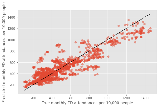
Model predicts monthly ED attendances per 10,000 people
To forecast raw numbers, need to multiply predicted value by population/10,000
def stacked_predict(X, models, m1_features, m2_features):

    rf1,rf2,final = models

    y_pred_1 = rf1.predict(X[m1_features])

    y_pred_2 = rf2.predict(X[m2_features])

    X_f = np.vstack([y_pred_1, y_pred_2]).T

    preds = final.predict(X_f)

    return preds
def forecast(data, pop, pop_g65, year, models, m1_features, m2_features):

    # model = reg

    data = data.merge(pop[[str(year),'ccg']],
                      left_on = 'ccg', right_on='ccg')

    data['population'] = data[str(year)]#*10000

    data = data.drop([str(year)],axis=1)

    data = data.merge(pop_g65[[str(year),'ccg']],
                      left_on = 'ccg', right_on='ccg')

    data['%>65'] = data[str(year)]*100/(data['population'])
    data['N>65'] = data[str(year)]

    X = data.drop(['ae_attendances_attendances','ccg',\
                   'month',str(year),'ccg'], axis=1)

    preds = stacked_predict(X, models, m1_features, m2_features)

    preds = preds*data['population'].values

    return preds
def sum_by_month(results):

    to_plot = []

    months = ['Jan','Feb','Mar','Apr','May','Jun',\
              'Jul','Aug','Sep','Oct','Nov','Dec']

    for month in months:

        res = results.loc[results.month==month]
        to_plot.append(np.mean(res[res.columns[2:]].values, axis=0))

    to_plot = np.array(to_plot).T

    points = []

    for row in to_plot:

        points.extend(row)

    return points
List to store scenario results#
scenario_results = []
Scaling factor for capacity increase#
F=1.1
Scenario 1: do nothing#
results = pd.DataFrame()
results['ccg'] = baseline['ccg']
results['month'] = baseline['month']
results['2019'] = baseline['ae_attendances_attendances']*baseline['population']

for year in np.arange(2020,2028):

    preds = forecast(baseline,population,pop_g65,year,models,m1_features,m2_features)

    results[str(year)] = preds
scenario_results.append(results)
Scenario 2: increase 111 capacity#
results = pd.DataFrame()
results['ccg'] = baseline['ccg']
results['month'] = baseline['month']
results['2019'] = baseline['ae_attendances_attendances']*baseline['population']

dta = baseline.copy()

for year in np.arange(2020,2028):

    dta['111_111_offered'] = baseline['111_111_offered'].values*F

    preds = forecast(dta,population,pop_g65,year,models,m1_features,m2_features)

    results[str(year)] = preds
scenario_results.append(results)
Scenario 3: increase 999 capacity#
results = pd.DataFrame()
results['ccg'] = baseline['ccg']
results['month'] = baseline['month']
results['2019'] = baseline['ae_attendances_attendances']*baseline['population']

dta = baseline.copy()

for year in np.arange(2020,2028):

    dta['amb_sys_answered'] = baseline['amb_sys_answered'].values*F

    preds = forecast(dta,population,pop_g65,year,models,m1_features,m2_features)

    results[str(year)] = preds
scenario_results.append(results)
Scenario 4: increase GP capacity#
results = pd.DataFrame()
results['ccg'] = baseline['ccg']
results['month'] = baseline['month']
results['2019'] = baseline['ae_attendances_attendances']*baseline['population']

dta = baseline.copy()

for year in np.arange(2020,2028):

    dta['gp_appt_available'] = baseline['gp_appt_available'].values*F

    preds = forecast(dta,population,pop_g65,year,models,m1_features,m2_features)

    results[str(year)] = preds
scenario_results.append(results)
Scenario 5: health of population at 2019#
results = pd.DataFrame()
results['ccg'] = baseline['ccg']
results['month'] = baseline['month']
results['2019'] = baseline['ae_attendances_attendances']*baseline['population']

dta = baseline.copy()


for year in np.arange(2020,2028):

    dta['People'] = [p+0.2 if p<np.mean(baseline.People.values) else p for p in dta.People.values]
    dta['Places'] = [p+0.2 if p<np.mean(baseline.Places.values) else p for p in dta.Places.values]
    dta['Lives'] = [p+0.2 if p<np.mean(baseline.Lives.values) else p for p in dta.Lives.values]

    preds = forecast(dta,population,pop_g65,year,models,m1_features,m2_features)

    results[str(year)] = preds
scenario_results.append(results)
Plot#
fig,ax = plt.subplots(figsize=(8,5))

scenarios = ['Population growth','111 capacity increase',
            'Ambulance capacity increase','GP capacity increase', 'Health of 2019']

for i,results in enumerate(scenario_results):

    if i==0:

        continue

    points = sum_by_month(results)

    points_series = pd.Series(points)

    plt.plot(np.arange(-12, 96),
             points_series.rolling(window=4).mean().to_list()[:],
             label = f'{scenarios[i]}')


points = sum_by_month(scenario_results[0])

points_series = pd.Series(points)

plt.plot(np.arange(-12, 96),
         points_series.rolling(window=4).mean().to_list()[:],
         'g--', label = f'{scenarios[0]}')


y = np.arange(24000,29000,1000)
plt.plot(np.zeros(len(y)),y, 'k--')

plt.legend(loc = 'lower left', fontsize=12)
plt.ylabel('Mean monthly ED attendances per CCG', fontsize=14)
plt.xlabel('Months since baseline', fontsize=14)
plt.xlim(0,48)

start, end = ax.get_xlim()
ax.xaxis.set_ticks(np.arange(-12, 50, 6))

plt.ylim(24500,28000)
plt.tight_layout()
plt.savefig('forecast_scaled.png', dpi=300)
plt.show()